Quickstart

In this first example, we will run a small ensemble of HOPS trajectories. Each trajectory in the ensemble represents the dynamics of an open quantum system for a given configuration of the environmental degrees of freedom. We begin with an open quantum systems Hamiltonian, represented as the sum of three pieces:

\[\hat{H} = \hat{H}_{\textrm{S}} + \sum_{n,q_n} \Lambda_{q_n} \hat{L}_n (\hat{a}^\dagger_{q_n} + \hat{a}_{q_n}) + \sum_{n,q_n} \hslash \omega_{q_n} (\hat{a}^\dagger_{q_n} \hat{a}_{q_n} + 1/2)\]

Where the first term (\(\hat{H}_S\)) is the system Hamiltonian, the second term represents the linear coupling between the system and each environmental degree of freedom, and the final term represents the thermal environment as a set of independent baths comprised of infinite harmonic oscillators.

For demonstration purposes we will run an ensemble of 100 trajectories to simulate the population dynamics of a molecular dimer. We will…

Build the trajectory by assigning parameters
Run the trajectory
Analyze the outcome

Creating the trajectory by assigning parameters

In order to create a trajectory, we will need to fill 5 dictionaries.

System_param: stores basic information about the system, bath, and system-bath coupling
Noise_param: specifies the generation of the noise
Eom_param: defines the equation of motion for time-evolving the hops trajectory
Integration_param: specifies characteristics of the integrator that time-evolves the hops trajectory via the equation of motion
Hierarchy_param: stores basic information about the hierarchy of auxiliary wave functions

There is also an optional dictionary where one can specify which data will be saved for analysis after code execution called storage_param.

After importing all the necessary libraries, we start by creating an empty list to store the system wave functions of all 100 trajectories.

import os
import numpy as np
import scipy as sp
from scipy import sparse
from pyhops.dynamics.hops_trajectory import HopsTrajectory as HOPS
from pyhops.dynamics.eom_hops_ksuper import _permute_aux_by_matrix
from pyhops.dynamics.bath_corr_functions import bcf_exp, bcf_convert_sdl_to_exp
import matplotlib.pyplot as plt

wf_list = []
ntraj = 100

First, we define the number of pigments in the linear chain we are simulating (nsite) and the system Hamiltonian matrix (hs).

In this example, each pigment in the aggregate has 2 adiabatic electronic states, a ground state \(\vert g \rangle\) and an excited state \(\vert e \rangle\). The basis for our system Hamiltonian is comprised of the diabatic electronic basis of local states. The system Hamiltonian is given by,

\[\hat{H}_{\textrm{S}} = \sum_n \vert n \rangle E_n \langle n \vert + \sum{n \neq m} \vert n \rangle V_{n,m} \langle m \vert\]

where, \(\vert n \rangle\) are the excited states of the pigments in the electronic system, \(E_n\) are the vertical excitation energies or the pigment energies, and \(V_{n,m}\) are the electronic couplings between pigments. The vertical excitation energies are the energy difference between the ground and first excited state of the pigment and are the diagonal elements of the system Hamiltonian. The electronic couplings are the off-diagonal values, such that the system Hamiltonian should be in this form given a 2-site system that consists of 2 coupled molecules.

\[\hat{H}_{\textrm{S}} = \begin{bmatrix} E_1 & V_{12}\\ V_{21} & E_2 \end{bmatrix}\]

In our example, the first and second molecules have vertical excitation energies of 100 and 0 wavenumbers, respectively. The coupling between the two sites (Hermitian-symmetric off-diagonals) is 50 wavenumbers. The system hamiltonian should then take the following array form:

\[\hat{H}_{\textrm{S}} = \begin{bmatrix} 100 & 50\\ 50 & 0 \end{bmatrix}\]

for trajectory_index in range(ntraj):
    nsite = 2
    hs = np.zeros([nsite, nsite])
    hs[0, 0] = 100
    hs[0, 1] = 50
    hs[1, 0] = 50
    hs[1, 1] = 0

Next, we describe the bath. The bath Hamiltonian describes the thermal environment surrounding the system. All of the vibrational degrees of freedom associated with a single pigment are combined into a single bath that is coupled to the electronic degrees of freedom of that pigment. In the HOPS formalism, the bath is an infinite set of coupled harmonic oscillators that mimic a continuous vibrational spectrum.

\[\hat{H}_{\textrm{B}} = \sum_{n,q_n} \hslash \omega_{q_n} (\hat{a}^\dagger_{q_n} \hat{a}_{q_n} + 1/2)\]

where \(\omega_{q_n}\) is the frequency of a harmonic oscillator and \(\hat{a}^\dagger_{q_n}\) and \(\hat{a}_{q_n}\) are the corresponding creation and annihilation operators. Each independent bath is indexed by \(n\) and contains a spectrum of harmonic modes indexed by \(q_n\).

The interaction Hamiltonian describes the coupling between the electronic degrees of freedom and the vibrational degrees of freedom. The interaction component is written as

\[\hat{H}_{\textrm{int}} = \sum_{n,q_n} \Lambda_{q_n} \hat{L}_n \hat{q}_n\]

Where \(\Lambda_{q_n}\) is a bi-linear coupling term and \(\hat{L}_n\) is an operator (in this case \(\hat{L}_n = \vert n\rangle{} \langle{} n \vert\)) that couples the \(n^{th}\) pigment to its independent environment described by bath modes \({q_n}\). We parametrize the bath and interaction Hamiltonians via a time correlation function and a set of L-operators.

The time correlation function of bath \(n\), \(C_n(t)\), is given in this example by an unshifted overdamped Drude-Lorentz model with a reorganization energy of 60 wavenumbers (e_lambda), reorganization timescale¹ of 60 wavenumbers (gamma), and temperature of 300 Kelvin (temp). The time correlation function governs the correlation of bath degrees of freedom, as well as the correlation of the noise trajectory.

In the HOPS formalism, a time correlation function must be represented as a sum of exponential modes: \(C_n(t) = \sum_{j_n}g_{j_n}e^{-w_{j_n}t/\hbar}\). We use the built-in bcf_convert_sdl_to_exp function to find the single-exponential form of the unshifted overdamped Drude-Lorentz time correlation function:

e_lambda = 60.0  
gamma = 60.0  
temp = 300.0  
(g_0, w_0) = bcf_convert_sdl_to_exp(e_lambda, gamma, 0.0, temp)

We now define our list of L-operators and match each with the exponential decomposition of the appropriate pigment’s correlation function: we will store these in lists of equal length, lop_list and gw_sysbath. We also apply a short time correction to the correlation function by implementing an additional mode for each pigment: we refer to this second mode as a Markovian mode. The Markovian mode is used to cancel the imaginary part of the correlation function at time 0 and disappears after a short time.

loperator = np.zeros([nsite, nsite, nsite], dtype=np.float64)  
gw_sysbath = []  
lop_list = []  
for i in range(nsite):  
    loperator[i, i, i] = 1.0  
    gw_sysbath.append([g_0, w_0])  
    lop_list.append(sp.sparse.coo_matrix(loperator[i]))  
    gw_sysbath.append([-1j * np.imag(g_0), 500.0])  
    lop_list.append(loperator[i]) 

We package all of our defined parameters into dictionaries so that we can later use them to create the trajectory object. See the linked chart for more details.

The sys_param dictionary takes:

a Hamiltonian matrix (HAMILTONIAN)
the exponential decomposition of the correlation function as a list of modes for the HOPS hierarchy and equation of motion (GW_SYSBATH) and the noise (PARAM_NOISE1)
the list of L operators for the HOPS hierarchy and equation of motion (L_HIER) and the noise (L_NOISE1)
the function that calculates the correlation function from an exponential mode at a given time (ALPHA_NOISE1).

sys_param = {
    "HAMILTONIAN": np.array(hs, dtype=np.complex128),  
    "GW_SYSBATH": gw_sysbath,  
    "L_HIER": lop_list,  
    "L_NOISE1": lop_list,
    "ALPHA_NOISE1": bcf_exp, 
    "PARAM_NOISE1": gw_sysbath, 
}

The noise dictionary takes:

a seed for the noise (SEED)
the noise model for producing correlated noise from a Gaussian white noise (MODEL)
the total time length of the noise trajectory in fs (TLEN)
the time-step resolution of the noise trajectory in fs (TAU).

Note that TLEN must be longer than the calculation is run for (the amount by which it is longer should correspond to the reorganization timescale).

noise_param = {
    "SEED": trajectory_index,
    "MODEL": "FFT_FILTER",
    "TLEN": 500.0,
    "TAU": 1.0, 
} 

Our calculation parameters consist of 3 small dictionaries describing the equation of motion (eom_param), integrator method (integrator_param), and hierarchy (hierarchy_param).

Equations of motion supported in this code include normalized nonlinear, linear, nonlinear, and nonlinear absorption. In this example, we are using a normalized nonlinear equation of motion as it allows for adaptivity in non-absorption calculations.

The integrator dictionary takes:

the type of integrator (INTEGRATOR). We currently only support a fourth-order Runge-Kutta integrator.

Other integrator parameters will be explored in the Adaptivity tutorial.

Lastly, hierarchy_param determines the triangular hierarchy truncation depth (MAXHIER) and also allows you to add static filters, which determines the structure of allowable hierarchy elements.

eom_param = {"EQUATION_OF_MOTION": "NORMALIZED NONLINEAR"}
integration_param = {"INTEGRATOR": "RUNGE_KUTTA"}   
hierarchy_param = {"MAXHIER": 4}

With all the parameters defined, we can finally create our HopsTrajectory object

hops = HOPS(
    sys_param,
    noise_param=noise_param,
    hierarchy_param=hierarchy_param,
    eom_param=eom_param,
    integration_param=integration_param,
)

Run the trajectory

Next, we will define our initial wave function (psi_0) and specify the time period over which the HOPS trajectory will propagate. In this example, we are fully populating site 0 and propagating the dynamics over 200 fs with a time step resolution of 4 fs. Finally, we avoid rounding errors by normalizing the wave function. Note that the integration time step must be an even integer multiple of TAU from noise_param.

psi_0 = np.array([0.0] * nsite, dtype=np.complex)
psi_0[0] = 1.0

psi_0 = psi_0 / np.linalg.norm(psi_0)

t_max = 200.0  
t_step = 4.0  

We will initialize HOPS trajectory with the initial wave function and propagate its dynamics.

hops.initialize(psi_0)
hops.propagate(t_max, t_step)

Analyze the outcome

We will save each physical wave function (hops.storage[‘psi_traj’]) in the wave function list.

psi_traj = hops.storage['psi_traj']
wf_list.append(psi_traj)

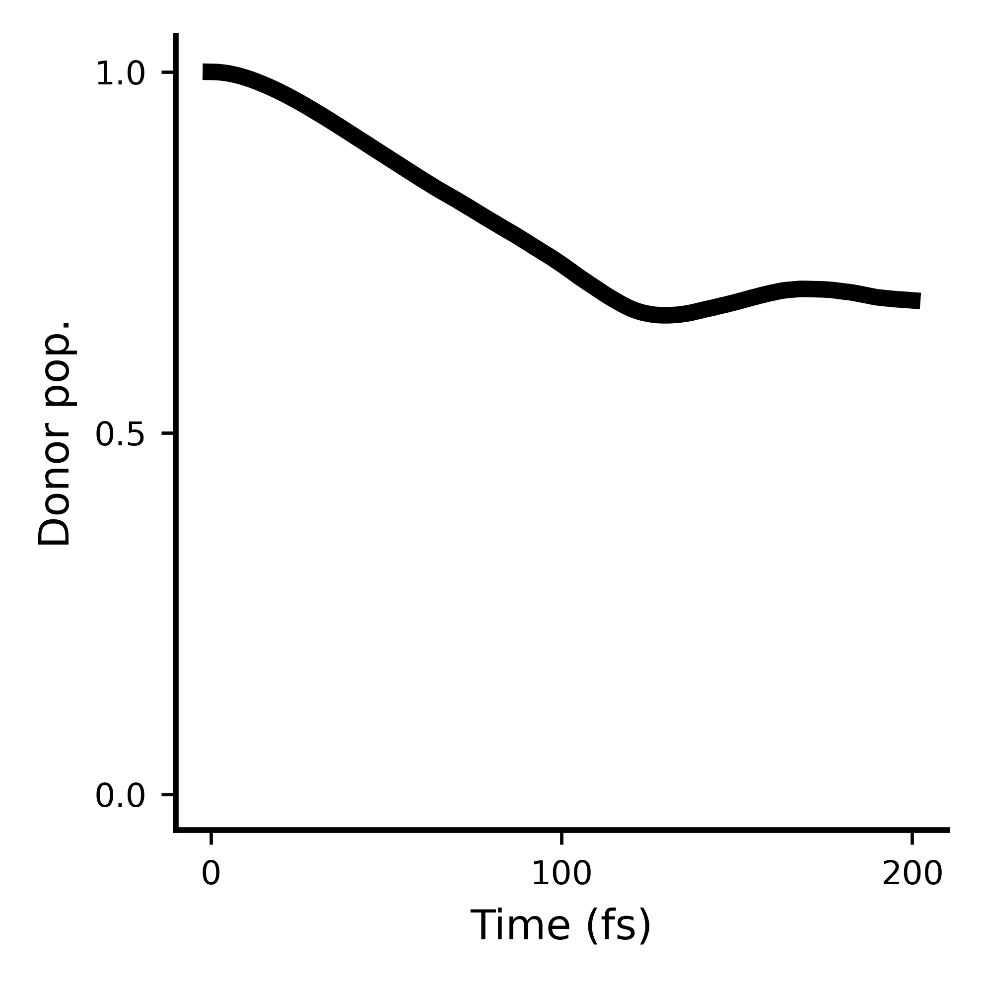
To plot the dynamics, we will make a plot of the mean population (absolute-square of the wave function) of the two sites over time.

mean_pop = np.mean(np.abs(np.array(wf_list))**2, axis=0)
pop1 = mean_pop[:,0]
pop2 = mean_pop[:,1]

t_axis = np.arange(0, t_max+t_step, t_step)
plt.xlabel("Time (fs)")
plt.ylabel("Population")
plt.plot(t_axis,pop1)
plt.plot(t_axis,pop2)
plt.show()

If done correctly, the results should look like this:

Graph

The full code to this example is shown below:

import os
import numpy as np
import scipy as sp
from scipy import sparse
from pyhops.dynamics.hops_trajectory import HopsTrajectory as HOPS
from pyhops.dynamics.eom_hops_ksuper import _permute_aux_by_matrix
from pyhops.dynamics.bath_corr_functions import bcf_exp, bcf_convert_sdl_to_exp
import matplotlib.pyplot as plt

wf_list = []
ntraj = 100

for trajectory_index in range(ntraj):

    nsite = 2
    hs = np.zeros([nsite, nsite])
    hs[0, 0] = 100
    hs[0, 1] = 50
    hs[1, 0] = 50
    hs[1, 1] = 0

    e_lambda = 60.0  
    gamma = 60.0  
    temp = 300.0  
    (g_0, w_0) = bcf_convert_sdl_to_exp(e_lambda, gamma, 0.0, temp)  

    loperator = np.zeros([nsite, nsite, nsite], dtype=np.float64)  
    gw_sysbath = []  
    lop_list = []  
    for i in range(nsite):  
        loperator[i, i, i] = 1.0  
        gw_sysbath.append([g_0, w_0])  
        lop_list.append(sp.sparse.coo_matrix(loperator[i]))  
        gw_sysbath.append([-1j * np.imag(g_0), 500.0])  
        lop_list.append(loperator[i]) 

    sys_param = {
        "HAMILTONIAN": np.array(hs, dtype=np.complex128),  
        "GW_SYSBATH": gw_sysbath,  
        "L_HIER": lop_list,  
        "L_NOISE1": lop_list,
        "ALPHA_NOISE1": bcf_exp, 
        "PARAM_NOISE1": gw_sysbath, 
    }

    noise_param = {
        "SEED": trajectory_index,
        "MODEL": "FFT_FILTER",
        "TLEN": 500.0,
        "TAU": 1.0, 
    } 

    eom_param = {"EQUATION_OF_MOTION": "NORMALIZED NONLINEAR"}
    integration_param = {"INTEGRATOR": "RUNGE_KUTTA"}   
    hierarchy_param = {"MAXHIER": 4}

    hops = HOPS(
        sys_param,
      noise_param=noise_param,
      hierarchy_param=hierarchy_param,
      eom_param=eom_param,
      integration_param=integration_param,
    )

    psi_0 = np.array([0.0] * nsite, dtype=np.complex)
    psi_0[0] = 1.0

    psi_0 = psi_0 / np.linalg.norm(psi_0)

    t_max = 200.0  
    t_step = 4.0  
    
    hops.initialize(psi_0)
    hops.propagate(t_max, t_step)

    psi_traj = hops.storage['psi_traj']
    wf_list.append(psi_traj)

mean_pop = np.mean(np.abs(np.array(wf_list))**2, axis=0)
pop1 = mean_pop[:,0]
pop2 = mean_pop[:,1]

t_axis = np.arange(0, t_max+t_step, t_step)
plt.xlabel("Time (fs)")
plt.ylabel("Population")
plt.plot(t_axis,pop1)
plt.plot(t_axis,pop2)
plt.show()

1: Also known as polaron formation timescale.