Adaptivity
The flagship feature of mesoHOPS is the adaptive Hierarchy of Pure States (adHOPS), a moving-basis construction of a HOPS calculation that achieves size-invariant scaling in large aggregates while remaining formally exact. By identifying the occupied system states and auxiliary wave functions and taking advantage of localization induced by the interaction of the system and bath to construct a time-evolving adaptive basis, adHOPS drastically reduces the basis size of a HOPS calculation and enables tractable simulations in systems that were previously too large to treat with an exact method of simulating open quantum systems.
In adaptive calculations, the HOPS object evaluates two types of errors at every basis update step: one associated with omitting each system state and auxiliary wave function currently in the basis, and the other linked to neglecting elements outside this basis. The basis then neglects its elements, beginning with those causing minimal error, until a designated derivative error boundary is met.
Given the full wave function \(\Psi_{t}\), the derivative error associated with transitioning to an adaptive basis (where \(\tilde{\Psi}_{t}\) represents the full wave function projected into the adaptive basis) must satisfy \(\left \Vert \frac{d\Psi_{t}}{dt} - \frac{d\tilde{\Psi}_{t}}{dt} \right \Vert_{2} \le \\delta\), where \(\delta\) is the user-defined error bound. Our state basis and auxiliary wave function basis are calculated separately with individual error bounds delta_a (\(\delta_A\)) and delta_s (\(\delta_S\)) such that \(\delta^2 = \delta_A^2 + \delta_S^2\).
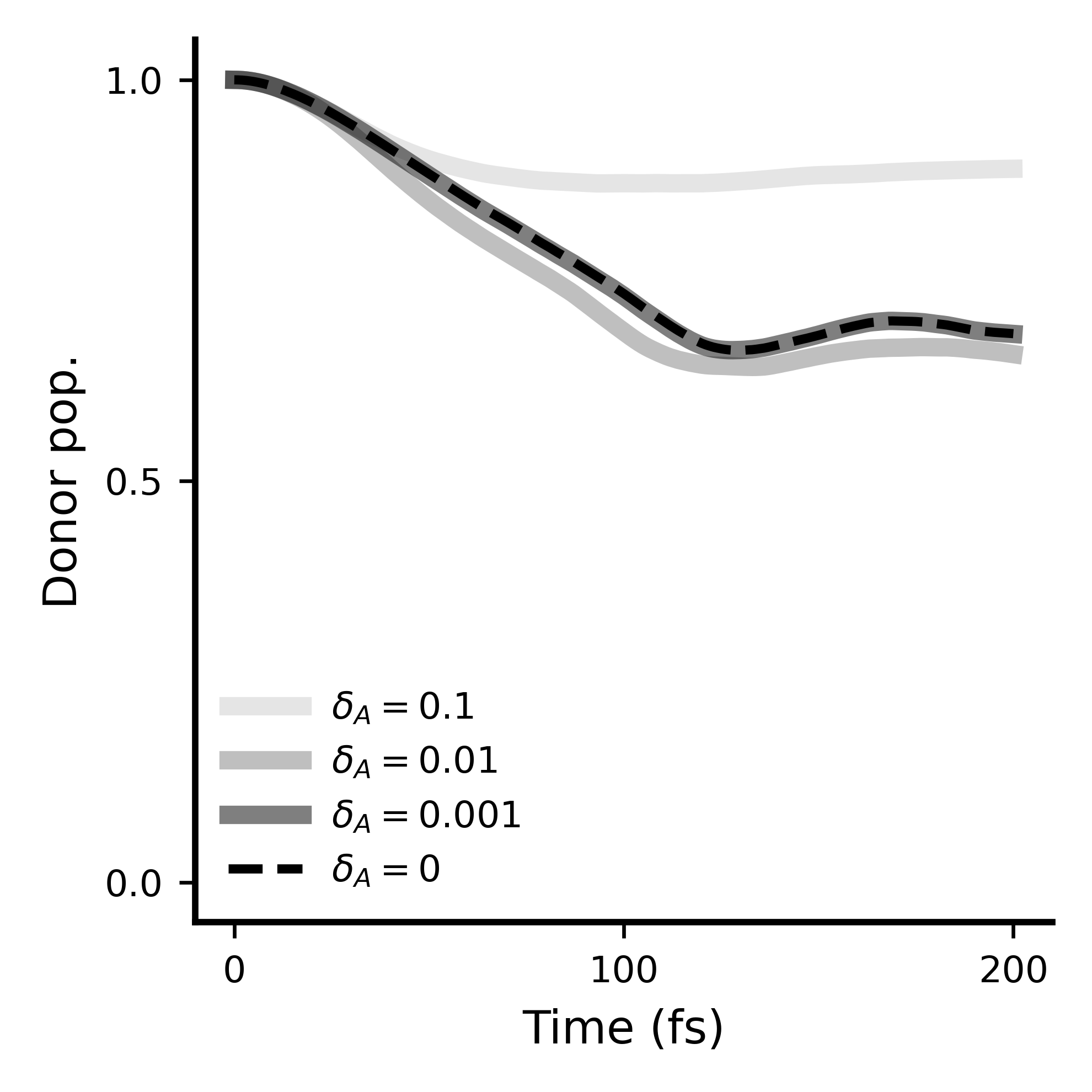
While there is no specific value of \(\delta\) for which the adaptive solution \(\tilde{\Psi}_{t}\) is guaranteed to converge to the non-adaptive solution \(\Psi_{t}\), we can run calculations with decreasing adaptivity parameter \(\delta\) until convergence is observed. This convergence has been demonstrated phenomenologically to be monotonic for \(\delta_A\), \(\delta_S\), and \(\delta\). As \(\delta \rightarrow 0\), the adaptive basis smoothly becomes the full basis defined by the system Hamiltonian, the correlation function modes, and the choice of hierarchy depth.
Because the adaptive basis rapidly expands at early times, constructing an appropriate basis can be challenging. There are three options for capturing the early-time dynamics of the adaptive basis: inchworm integration,static basis definition, and hierarchy inchworm integration. We call these the early adaptive integrators.
When creating a HOPS trajectory, we can specify our choice of early adaptive integrator as well as other parameters for the early-time integration in adaptive HOPS calculations in the integrator_param dictionary.
When doing adaptive HOPS calculations, this dictionary should contain:
- The type of integrator (INTEGRATOR). We currently only support a fourth-order Runge-Kutta integrator (RUNGE_KUTTA).
- The type of early adaptive integrator (EARLY_ADAPTIVE_INTEGRATOR). We currently support inchworm (INCH_WORM), static (STATIC), and hierarchy inchworm (STATIC_STATE_INCHWORM_HIERARCHY).
- Inchworm early integration ensures that the basis grows aggressively by recalculating the basis multiple times at each early time step.
- Static early integration allows the user to define the basis at early time.
- Hierarchy inchworm early integration allows the user to define the state basis as a static basis, but calculates the auxiliary wave function basis through inchworm integration.
- The number of timesteps defining early time (EARLY_INTEGRATOR_STEPS)
If we choose inchworm or hierarchy inchworm as our early adaptive integrator, we need to also specify:
- The number of times the adaptive basis is recalculated to account for the rapid growth at early time before time-evolving the dynamics (INCHWORM_CAP)
Example of the resulting integration_params:
integration_param = {"INTEGRATOR": "RUNGE_KUTTA",
                         "EARLY_ADAPTIVE_INTEGRATOR": "INCH_WORM",
                         "EARLY_INTEGRATOR_STEPS": 5,
                         "INCHWORM_CAP" : 5,
 "STATIC_BASIS": None}
Note that we can also specify the static basis when using inchworm integration but this will result in the static basis being the basis at the initial time.
If we choose to define our static basis, we need to also specify:
- The static basis during early time (STATIC_BASIS)
Example of the resulting integration_params:
integration_param = {"INTEGRATOR": "RUNGE_KUTTA",
                         "EARLY_ADAPTIVE_INTEGRATOR": "STATIC",
                         "EARLY_INTEGRATOR_STEPS": 5,
                         "STATIC_BASIS" : [state_list, aux_list]}
The make_adaptive(delta_a, delta_s, update_step) method must be called before the initialization of the trajectory and after creating the HOPs trajectory to implement a moving, adaptive basis guaranteed to satisfy derivative error bound delta. Adaptivity parameters delta_a (\(\delta_A\)) and delta_s (\(\delta_S\)) control the sensitivity of the adaptive basis construction and update_step is the parameter that determines how often the adaptive HOPS basis will be updated.
Example of the make_adaptive function:
delta_s = 0
delta_a = 0.001
update_step = 10
hops.make_adaptive(delta_a, delta_s, update_step)
If done correctly, the results should look like this (for the shown values of delta_a (\(\delta_A\))):